Examining U.S. radio antenna locations with Tableau Desktop 9
For today’s demo I’m going to parse a data.gov file that contains U.S. radio tower locations into a cool map figure. I’ll be using Apache Drill to handle reading in and manipulating the geographic coordinate fields in the file, and Tableau Desktop 9 to provide an easy way to generate a map based on the data.
Attaching Tableau to Drill data in Microsoft Windows is pretty easy. Assuming you already have Drill (see this article) and Tableau installed, you just need to download and install this ODBC driver from MapR (choose the 64-bit .msi file). That’s all you’ll need to be able to follow along with this demo, so let’s turn our attention back to the data.
Go ahead and download the zipped antenna files located on this site. Once they’re unzipped, rename the ‘CO.dat’ file to 'CO.tbl’ (be sure to turn on 'File name extensions’ under 'View’). This renaming tells Drill to use the pipe symbol ’|’ as a delimiter for columns in the file.
So let’s take a look at the data:
> SELECT * FROM dfs.`C:\Path\To\r_tower\CO.tbl` LIMIT 10;
+-----------------------------------------------------------------------------------------------------------------------+
|                                                        columns                                                        |
+-----------------------------------------------------------------------------------------------------------------------+
| ["CO","REG","A0925026","1293612","2693131","T","","","","","","","","","","","","\r"]                                 |
| ["CO","REG","A0971560","1295891","2695410","T","","","","","","","","","","","","\r"]                                 |
| ["CO","REG","A0977407","1296672","2696191","T","","","","","","","","","","","","\r"]                                 |
| ["CO","REG","A0980840","1297184","2696703","T","","","","","","","","","","","","\r"]                                 |
| ["CO","REG","A0000039","1000019","96973","T","41","9","58.0","N","148198.0","81","15","23.0","W","292523.0","","\r"]  |
| ["CO","REG","A0000069","1000042","96980","T","32","40","31.0","N","117631.0","97","8","29.0","W","349709.0","","\r"]  |
| ["CO","REG","A0000072","1000044","96982","T","32","53","2.0","N","118382.0","96","48","34.0","W","348514.0","","\r"]  |
| ["CO","REG","A0000073","1000045","96983","T","32","57","6.0","N","118626.0","97","3","52.0","W","349432.0","","\r"]   |
| ["CO","REG","A0000097","1000064","96988","T","33","36","0.0","N","120960.0","85","50","0.0","W","309000.0","","\r"]   |
| ["CO","REG","A0000122","1000086","96991","T","25","51","59.0","N","93119.0","80","17","6.0","W","289026.0","","\r"]   |
+-----------------------------------------------------------------------------------------------------------------------+
Looks like we have a couple quirks to do deal with: 1.) the latitude and longitude information is spread across several columns and represented in sexigesimal format (see this Wiki link), and 2.) at least some geographic fields are blank, so we’ll need to account for that when we process the file.
After some thought (and trial and error), I came up with following 'antenna’ view to hold the geo data that we want to access from Tableau:
CREATE VIEW antennas AS
     SELECT CAST(columns[6] AS FLOAT)+(CAST(columns[7] AS FLOAT)/60)+(CAST(columns[8] AS FLOAT)/3600) lat,
            -1*(CAST(columns[11] AS FLOAT)+(CAST(columns[12] AS FLOAT)/60)+(CAST(columns[13] AS FLOAT)/3600)) long
       FROM dfs.`C:\Path\To\r_tower\CO.tbl`
      WHERE LENGTH(columns[6]) > 0;
But please note: Before you issue this command you should switch to a writable schema by entering:
USE dfs.tmp;
Now that the view is created, we can focus on connecting Tableau to Drill and loading in the data. With Drill still running in a Command Prompt window, launch Tableau and select “More Servers…” from the “Connect” panel on the left-hand side. Then click “Other Databases (ODBC).” In the dialog box that appears, select “MapR ODBC Driver for Drill DSN” next to the “DSN” radio button. Now click “Connect”, then “OK” in the new window that pops up, followed by “OK” in the original window.
With the connection to Drill completed, we can start hunting for our data. Type 'dfs.tmp’ into the 'Schema’ dropdown on the left and then select it. Now do the same for the Table dropdown below it, but this time type in the name of our view, “antennas.” Now drag the 'antennas’ table that appears below into the big blank space that says 'Drag tables here.’ Now it’s time to tell Tableau that 'Long’ entries are actually 'longitude,’ so click the hash symbol next to the label down below and select “Longitude” from the “Geographic Role” submenu. To begin making our map figure, click “Sheet 1” in the lower left of the window.
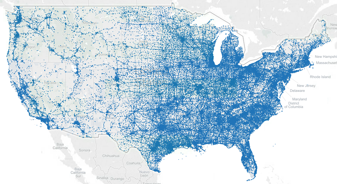
On this screen drag “Lat” from under “Measures” on the left to “Rows” up top, and then perform a similar operation for “Long” and “Columns.” Now hit the small down-arrow next to the newly created row and column entries of 'AVG(Lat)’ and 'AVG(Long),’ changing their types from 'Measure (Average)’ to 'Dimension.’ And that’s it! You should now be looking at a map of antenna locations in the United States that you can zoom and pan.

Locations of radio towers within the continental United States.
Pretty neat! This plot definitely explains some of the issues I had with cell coverage last time I drove across the Western states.
Even though this is a simple demo, you can really see how using Drill to process data and Tableau to visualize it plays to the strengths of both pieces of software. It’s a potent combination, and one you should definitely look into using if you’re doing analytic work.